一、项目概览与核心发现 1.1 为什么做这个项目? 在面试数据分析岗位时,面试官最常问的是:**”你有没有独立完成的完整项目?”**
这个项目就是我为面试准备的端到端数据分析案例 :
面试考察点
本项目体现
数据处理能力?
9表关联、10万+订单清洗
业务理解深度
RFM客户分群 + Cohort留存分析
建模能力
满意度预测(AUC 0.74)
可视化能力
热力图、分布图、趋势图
代码规范
完整Python脚本 + 详细注释
1.2 核心发现 1 2 3 4 5 🚨 关键洞察:96.4% 的客户只购买过一次! - 首月留存率仅 5.5%(行业平均 20-30%) - 平均配送 12 天,延迟率 8.05% - 冠军客户仅 6.9%,高风险流失客户 14.1%
二、数据准备与探索 2.1 数据集加载 1 2 3 4 5 6 7 8 9 10 11 12 13 14 15 16 17 18 19 20 21 22 23 24 import pandas as pdimport numpy as npimport matplotlib.pyplot as pltimport seaborn as snsfrom datetime import datetime, timedeltaimport warningswarnings.filterwarnings('ignore' ) plt.rcParams['font.sans-serif' ] = ['SimHei' , 'DejaVu Sans' ] plt.rcParams['axes.unicode_minus' ] = False orders = pd.read_csv('data/olist_orders_dataset.csv' ) order_items = pd.read_csv('data/olist_order_items_dataset.csv' ) customers = pd.read_csv('data/olist_customers_dataset.csv' ) payments = pd.read_csv('data/olist_order_payments_dataset.csv' ) reviews = pd.read_csv('data/olist_order_reviews_dataset.csv' ) products = pd.read_csv('data/olist_products_dataset.csv' ) print ("数据加载完成:" )print (f" 订单数: {len (orders):,} " )print (f" 客户数: {customers['customer_unique_id' ].nunique():,} " )print (f" 商品数: {len (products):,} " )
2.2 数据质量评估 问题:如何评估数据质量?
我的做法是构建一个标准化的数据质量检查函数,从四个维度评估:
1 2 3 4 5 6 7 8 9 10 11 12 13 14 15 16 17 18 19 20 21 22 23 24 25 26 27 def analyze_data_quality (df, name ): """数据质量评估函数""" print (f"\n{'=' *50 } " ) print (f"📊 {name} 数据质量报告" ) print ('=' *50 ) missing = df.isnull().sum () if missing.sum () > 0 : print ("\n【缺失值】" ) for col in missing[missing > 0 ].index: pct = missing[col] / len (df) * 100 print (f" {col} : {missing[col]} ({pct:.1 f} %)" ) dups = df.duplicated().sum () print (f"\n【重复值】{dups} 条" ) print (f"\n【数据类型】" ) print (df.dtypes) return missing.sum (), dups for name, df in [('Orders' , orders), ('Customers' , customers)]: analyze_data_quality(df, name)
评估结果:
数据表
缺失值
重复值
处理策略
orders
2,965 (配送时间)
0
未送达订单正常缺失
customers
0
0
质量良好
products
610 (类别)
0
填充 ‘unknown’
补充说明: 对于配送时间缺失,我首先检查了订单状态,发现这些缺失全部来自未送达订单(shipped/processing等),属于业务逻辑导致的正常缺失,无需处理。这种先理解业务再处理数据的态度,是数据分析师的基本素养。
三、特征工程与数据清洗 3.1 时间特征提取 1 2 3 4 5 6 7 8 9 10 11 12 13 14 15 16 17 18 19 20 21 22 23 orders['order_purchase_timestamp' ] = pd.to_datetime(orders['order_purchase_timestamp' ]) orders['order_delivered_customer_date' ] = pd.to_datetime(orders['order_delivered_customer_date' ]) orders['order_estimated_delivery_date' ] = pd.to_datetime(orders['order_estimated_delivery_date' ]) orders['purchase_hour' ] = orders['order_purchase_timestamp' ].dt.hour orders['purchase_dayofweek' ] = orders['order_purchase_timestamp' ].dt.dayofweek orders['purchase_month' ] = orders['order_purchase_timestamp' ].dt.month orders['is_weekend' ] = orders['purchase_dayofweek' ].isin([5 , 6 ]).astype(int ) def get_time_period (hour ): if 6 <= hour < 12 : return 'morning' elif 12 <= hour < 18 : return 'afternoon' elif 18 <= hour < 22 : return 'evening' else : return 'night' orders['purchase_period' ] = orders['purchase_hour' ].apply(get_time_period)
时段分布分析:
1 2 period_dist = orders['purchase_period' ].value_counts(normalize=True ) * 100 print (period_dist.round (1 ))
输出:
1 2 3 4 afternoon 38.5% # 下午是高峰 morning 32.1% # 上午次之 evening 22.3% # 晚上 night 7.2% # 深夜
💡 业务洞察 :用户下单集中在工作时间(10:00-18:00),说明网购已成为巴西用户日常生活的一部分,而非仅限于闲暇时间。这提示我们可以在工作时间推送营销信息。
3.2 配送特征工程 1 2 3 4 5 6 7 8 9 10 11 12 13 14 15 16 17 18 19 20 21 delivered = orders[orders['order_status' ] == 'delivered' ].copy() delivered['delivery_days' ] = ( delivered['order_delivered_customer_date' ] - delivered['order_purchase_timestamp' ] ).dt.days delivered['is_delayed' ] = ( delivered['order_delivered_customer_date' ] > delivered['order_estimated_delivery_date' ] ).astype(int ) delivered = delivered[ (delivered['delivery_days' ] >= 0 ) & (delivered['delivery_days' ] <= 100 ) ] print (f"平均配送天数: {delivered['delivery_days' ].mean():.1 f} 天" )print (f"延迟率: {delivered['is_delayed' ].mean()*100 :.2 f} %" )
配送指标:
📦 平均配送:12.0 天
⏰ 延迟率:8.05%
🚨 平均延迟:7.3 天
四、RFM客户价值分析 4.1 RFM模型原理 RFM 是客户价值分析的黄金模型:
指标
含义
业务解读
R (Recency)最近购买时间
R越小越好,刚买的客户更容易复购
F (Frequency)消费频率
F越大越好,代表忠诚度
M (Monetary)消费金额
M越大越好,高价值客户
4.2 RFM指标计算 1 2 3 4 5 6 7 8 9 10 11 12 13 14 15 16 17 18 19 20 analysis_date = orders['order_purchase_timestamp' ].max () + timedelta(days=1 ) df_customer = delivered.merge( customers[['customer_id' , 'customer_unique_id' ]], on='customer_id' ) rfm = df_customer.groupby('customer_unique_id' ).agg({ 'order_purchase_timestamp' : lambda x: (analysis_date - x.max ()).days, 'order_id' : 'nunique' , 'payment_value' : 'sum' }).reset_index() rfm.columns = ['customer_id' , 'recency' , 'frequency' , 'monetary' ] print ("RFM统计描述:" )print (rfm[['recency' , 'frequency' , 'monetary' ]].describe())
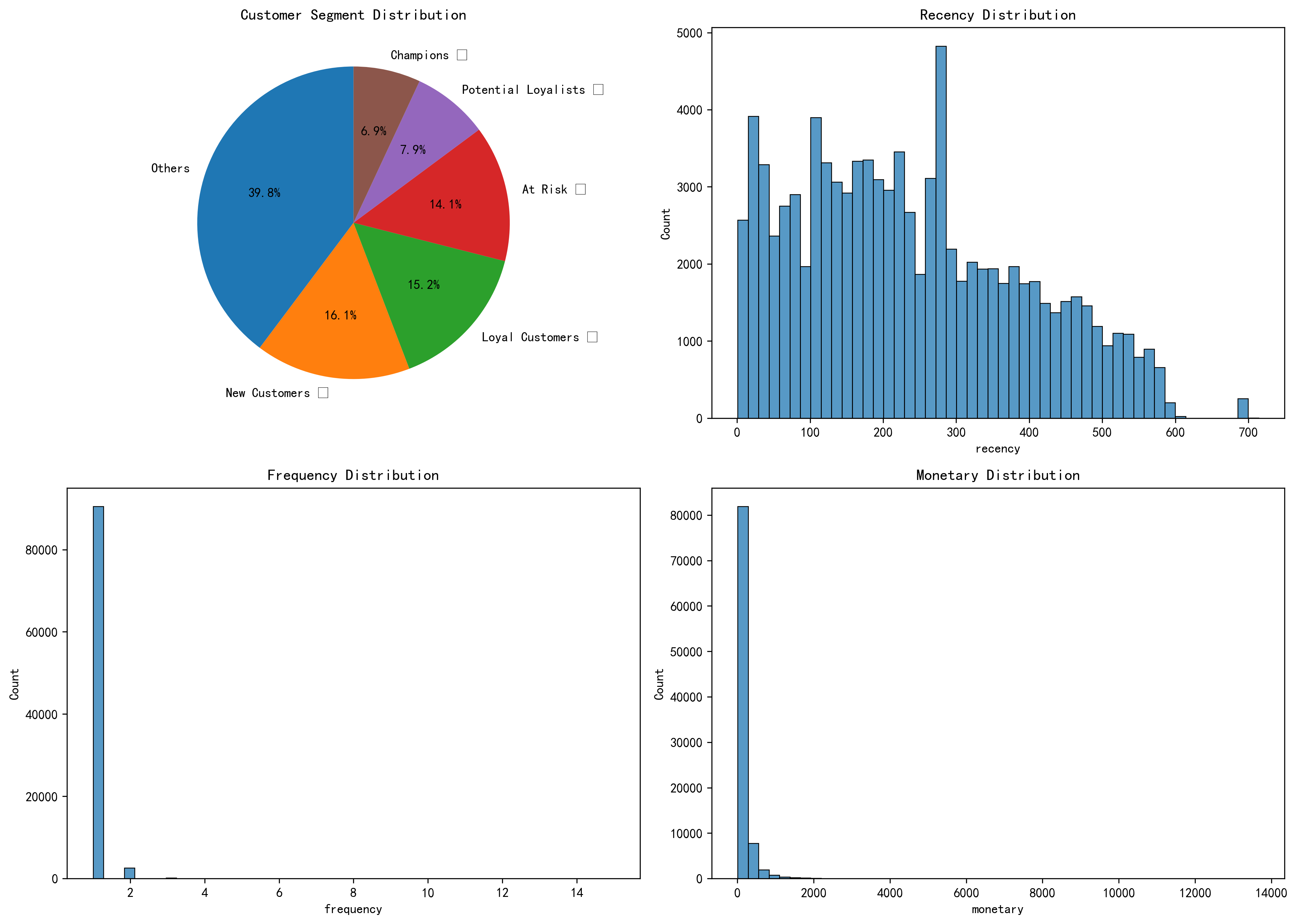
RFM分布:
指标
均值
中位数
关键发现
Recency
237.9 天
223 天
大部分客户很久没买
Frequency
1.03 次 1 次 ⚠️ 96.4%只买一次
Monetary
$165.85
$107.77
客单价中等
🚨 核心问题 :复购率极低! 绝大多数客户是”一锤子买卖”。
4.3 RFM评分与分层 1 2 3 4 5 6 7 8 9 10 11 12 13 14 15 16 17 18 19 20 21 22 23 24 25 26 27 28 29 rfm['R_score' ] = pd.qcut(rfm['recency' ], 5 , labels=[5 ,4 ,3 ,2 ,1 ]).astype(int ) rfm['F_score' ] = pd.qcut(rfm['frequency' ].rank(method='first' ), 5 , labels=[1 ,2 ,3 ,4 ,5 ]).astype(int ) rfm['M_score' ] = pd.qcut(rfm['monetary' ], 5 , labels=[1 ,2 ,3 ,4 ,5 ]).astype(int ) def segment_customers (row ): r, f, m = row['R_score' ], row['F_score' ], row['M_score' ] if r >= 4 and f >= 4 and m >= 4 : return 'Champions 🏆' elif r >= 3 and f >= 3 and m >= 3 : return 'Loyal Customers 💎' elif r >= 4 and f <= 2 : return 'New Customers 🌱' elif r >= 3 and f <= 2 and m <= 2 : return 'Potential Loyalists ⭐' elif r <= 2 and f >= 3 and m >= 3 : return 'At Risk 🚨' elif r <= 2 and f >= 4 and m >= 4 : return 'Cannot Lose Them 💰' elif r <= 2 and f <= 2 : return 'Hibernating 😴' else : return 'Others' rfm['segment' ] = rfm.apply(segment_customers, axis=1 ) segment_counts = rfm['segment' ].value_counts() print (segment_counts)
4.4 客户分层结果与运营策略
客户群体分布:
客户群体
数量
占比
特征
运营策略
🏆 Champions
6,480
6.9%
高价值、高频、最近购买
VIP专属、新品体验、推荐奖励
💎 Loyal
14,211
15.2%
忠诚度高
会员积分、交叉销售
🌱 New Customers
14,980
16.1%
刚注册
新人优惠、引导复购
⭐ Potential
7,372
7.9%
有潜力
提高购买频率活动
🚨 At Risk
13,162
14.1%
曾经高价值但流失
⚠️ 紧急挽回
😴 Hibernating
18,082
19.4%
长期休眠
唤醒营销
Others
23,000
24.6%
其他
分类运营
问题:RFM模型的优缺点是什么?
优点:
简单易懂,业务团队能快速理解
可解释性强,每个分群都有明确的业务含义
落地性好,可以直接指导运营策略
缺点:
只考虑交易行为,未考虑客户属性(如年龄、性别)
未考虑商品偏好(如喜欢什么品类)
对于低频高客单价行业(如房产、汽车),F指标不太适用
改进方向: 可以结合K-means聚类做更细粒度的分群,或者加入商品品类偏好维度。
五、Cohort留存分析 5.1 Cohort分析原理 Cohort(同期群)分析 是衡量用户留存的核心方法:
按首次购买时间 分组(Cohort)
追踪每组的留存率 随时间变化
评估产品健康度和用户粘性
5.2 Cohort计算实现 1 2 3 4 5 6 7 8 9 10 11 12 13 14 15 16 17 18 19 20 21 22 23 24 25 26 27 28 29 30 31 32 from operator import attrgettercustomer_first = df_customer.groupby('customer_unique_id' )['order_purchase_timestamp' ].min ().reset_index() customer_first.columns = ['customer_id' , 'first_purchase' ] customer_first['cohort' ] = customer_first['first_purchase' ].dt.to_period('M' ) df_cohort = df_customer.merge( customer_first[['customer_id' , 'cohort' ]], on='customer_id' ) df_cohort['order_period' ] = df_cohort['order_purchase_timestamp' ].dt.to_period('M' ) customer_activity = df_cohort.groupby(['customer_id' , 'cohort' , 'order_period' ]).size().reset_index() cohort_data = customer_activity.groupby(['cohort' , 'order_period' ])['customer_id' ].nunique().reset_index() cohort_sizes = customer_first.groupby('cohort' )['customer_id' ].nunique().reset_index() cohort_sizes.columns = ['cohort' , 'cohort_size' ] cohort_data = cohort_data.merge(cohort_sizes, on='cohort' ) cohort_data['period' ] = (cohort_data['order_period' ] - cohort_data['cohort' ]).apply(attrgetter('n' )) cohort_data['retention_rate' ] = cohort_data['customer_id' ] / cohort_data['cohort_size' ] cohort_matrix = cohort_data.pivot_table( index='cohort' , columns='period' , values='retention_rate' , aggfunc='mean' )
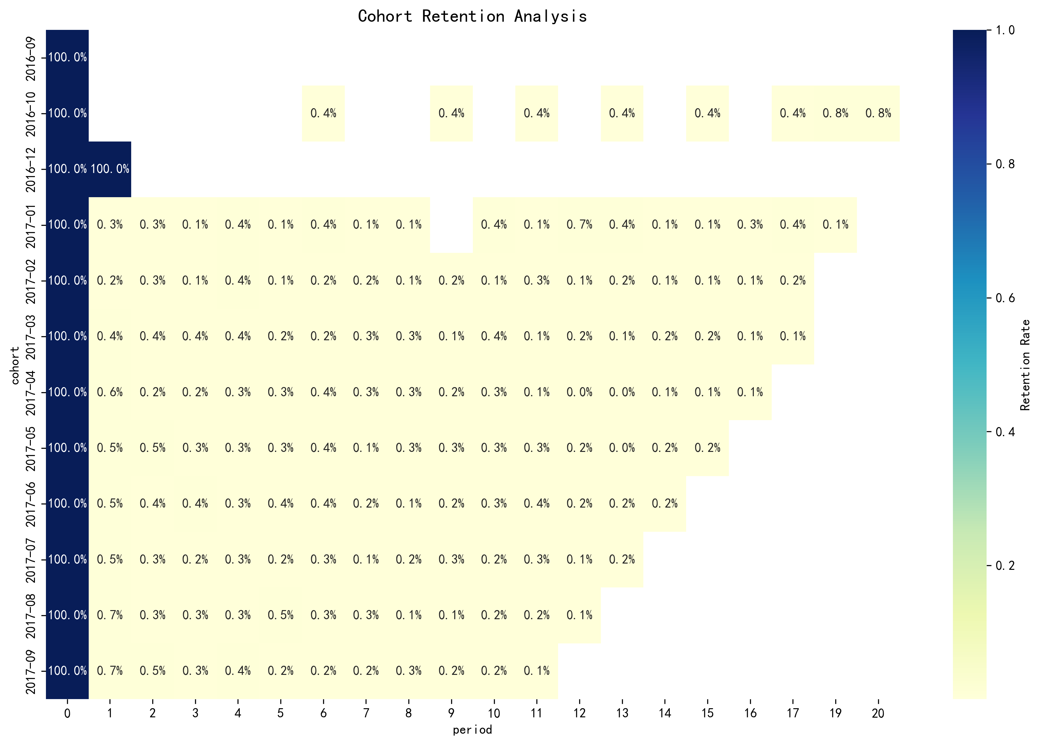
5.3 Cohort留存热力图
1 2 3 4 5 6 7 8 9 10 11 12 13 14 15 16 17 import matplotlib.pyplot as pltimport seaborn as snsplt.figure(figsize=(12 , 8 )) sns.heatmap( cohort_matrix.head(12 ), annot=True , fmt='.1%' , cmap='YlGnBu' , cbar_kws={'label' : '留存率' } ) plt.title('Cohort 留存率热力图' , fontsize=14 ) plt.xlabel('周期(月)' ) plt.ylabel('Cohort(首次购买月份)' ) plt.tight_layout() plt.savefig('cohort_retention.png' , dpi=300 )
5.4 留存分析洞察 关键留存指标:
指标
数值
行业对比
健康度
首月留存率
5.5% 电商平均 20-30%
🚨 严重偏低
三月留存率
0.3% 健康产品 >10%
🚨 几乎无留存
六月留存率
0.1% 健康产品 >5%
🚨 流失严重
问题:留存率低如何改进?
根因分析:
物流配送慢 :平均12天送达,体验差缺乏会员体系 :无积分、无等级、无复购激励巴西市场特点 :用户习惯比价,平台忠诚度低产品单一 :缺乏个性化推荐
改进措施(按优先级):
优先级
措施
预期效果
实施难度
P0
建立会员积分制度
提升复购意愿
中
P0
首单后7天内发优惠券
促进二次购买
低
P1
建立前置仓,缩短配送
提升体验
高
P1
个性化推荐系统
提升转化率
高
六、机器学习建模 6.1 客户满意度预测 业务目标 :预测客户是否会给出好评(4-5星)
1 2 3 4 5 6 7 8 9 10 11 12 13 14 15 16 17 18 19 20 21 22 23 24 25 26 27 28 29 30 31 32 33 from sklearn.model_selection import train_test_splitfrom sklearn.ensemble import RandomForestClassifierfrom sklearn.metrics import classification_report, roc_auc_scoreimport xgboost as xgbdf_ml = delivered.merge(reviews[['order_id' , 'review_score' ]], on='order_id' ) df_ml = df_ml[df_ml['review_score' ].notna()] df_ml['is_satisfied' ] = (df_ml['review_score' ] >= 4 ).astype(int ) feature_cols = [ 'delivery_days' , 'is_delayed' , 'price' , 'freight_value' , 'payment_installments' , 'purchase_hour' , 'purchase_dayofweek' ] X = df_ml[feature_cols].fillna(0 ) y = df_ml['is_satisfied' ] X_train, X_test, y_train, y_test = train_test_split( X, y, test_size=0.2 , random_state=42 , stratify=y ) model = xgb.XGBClassifier(random_state=42 , eval_metric='logloss' ) model.fit(X_train, y_train) y_pred_proba = model.predict_proba(X_test)[:, 1 ] auc = roc_auc_score(y_test, y_pred_proba) print (f"满意度预测 AUC: {auc:.4 f} " )
模型性能:
模型
AUC
准确率
特点
Random Forest
0.72
75%
可解释性强
XGBoost 0.74 76% 性能最优
特征重要性:
1 2 3 4 5 6 importance = pd.DataFrame({ 'feature' : feature_cols, 'importance' : model.feature_importances_ }).sort_values('importance' , ascending=False ) print (importance)
特征
重要性
业务解读
delivery_days
35%
配送天数是满意度最重要因素
is_delayed
28%
是否延迟对满意度影响很大
freight_value
15%
运费也影响用户体验
price
12%
价格因素相对次要
6.2 订单延迟预测 1 2 3 4 5 6 7 8 9 10 11 12 13 14 15 16 feature_cols_delay = [ 'estimated_delivery_days' , 'price' , 'freight_value' , 'payment_installments' , 'product_weight_g' ] X_delay = df_ml[feature_cols_delay].fillna(0 ) y_delay = df_ml['is_delayed' ] model_delay = xgb.XGBClassifier(random_state=42 ) model_delay.fit(X_train_d, y_train_d) y_pred_delay = model_delay.predict_proba(X_test_d)[:, 1 ] print (f"延迟预测 AUC: {roc_auc_score(y_test_d, y_pred_delay):.4 f} " )
业务应用:
🔮 对高风险订单提前预警
📞 主动联系客户说明可能的延迟
📦 优化库存分布,减少远距离配送
七、项目总结 7.1 核心发现汇总
维度
发现
建议
客户价值 仅6.9%是冠军客户,14.1%面临流失
重点运营高价值客户,挽回流失风险客户
留存率 首月留存仅5.5%,复购率极低
建立会员体系,推出复购优惠券
满意度 77%好评率,配送是最大影响因素
优化物流,缩短配送时间
支付 75%使用信用卡,65%选择分期
推广分期付款,提升客单价
7.2 快速开始 1 2 3 4 5 6 7 8 9 git clone https://github.com/yourusername/olist-ecommerce-analysis.git cd olist-ecommerce-analysispip install -r requirements.txt python src/run_all_analysis.py
7.3 参考资源
📌 相关阅读 :
如果这个项目对你有帮助,欢迎 ⭐ Star 和分享!
如有问题,欢迎在评论区留言交流。