均值方差模型图片

均值方差模型

代码如下：
import pandas as pd
import numpy as np
import scipy.optimize as sco
import matplotlib.pyplot as plt

# ====================== 1. 内嵌模拟A股数据 ======================
np.random.seed(42)  # 固定随机种子，结果可复现
# 标的信息（A股）
tickers = ['600519.SH', '300750.SZ', '600036.SH', '002594.SZ', '000651.SZ']
ticker_names = ['贵州茅台', '宁德时代', '招商银行', '比亚迪', '格力电器']
name_map = dict(zip(tickers, ticker_names))

# 生成5年日频收盘价（252*5=1260个交易日）
n_days = 252 * 5
base_prices = [1000, 200, 30, 150, 30]  # 初始股价（贴合A股真实价格）
prices_data = []
for i in range(len(tickers)):
    # 模拟日收益率（均值0.03%，波动率1.5%，贴合A股特征）
    daily_ret = np.random.normal(0.0003, 0.015, n_days)
    # 计算累计收益率 -> 收盘价
    cum_ret = np.cumprod(1 + daily_ret)
    price_series = base_prices[i] * cum_ret
    prices_data.append(price_series)

# 构建价格DataFrame
prices = pd.DataFrame(
    np.array(prices_data).T,
    columns=tickers,
    index=pd.date_range(start='2019-01-01', periods=n_days, freq='B')  # B=工作日
)

# 计算日对数收益率（剔除首行缺失值）
daily_returns = np.log(prices / prices.shift(1)).dropna()

# ====================== 2. 均值方差模型核心逻辑 ======================
# 年化预期收益率（日均值 * 252）
mu = daily_returns.mean() * 252
# 年化协方差矩阵（日协方差 * 252）
cov = daily_returns.cov() * 252
# 无风险利率（国内1年期国债收益率，取2%）
risk_free_rate = 0.02

# 定义组合收益/风险/夏普比率计算函数
def portfolio_performance(weights, mu, cov):
    port_return = np.sum(mu * weights)  # 组合收益
    port_vol = np.sqrt(np.dot(weights.T, np.dot(cov, weights)))  # 组合波动率
    sharpe_ratio = (port_return - risk_free_rate) / port_vol  # 夏普比率
    return port_return, port_vol, sharpe_ratio

# 优化目标1：最小化组合波动率（用于有效前沿/最小方差组合）
def minimize_volatility(weights, mu, cov):
    return portfolio_performance(weights, mu, cov)[1]

# 优化目标2：最大化夏普比率（等价于最小化负夏普比率）
def maximize_sharpe(weights, mu, cov):
    return -portfolio_performance(weights, mu, cov)[2]

# 约束条件：权重和为1；边界：权重∈[0,1]（不允许做空）
constraints = ({'type': 'eq', 'fun': lambda x: np.sum(x) - 1})
bounds = tuple((0, 1) for _ in range(len(tickers)))
initial_guess = np.array([1/len(tickers)] * len(tickers))  # 等权初始值

# 2.1 最小方差组合（风险最低）
min_vol_result = sco.minimize(
    minimize_volatility, initial_guess,
    args=(mu, cov), method='SLSQP',
    bounds=bounds, constraints=constraints
)
min_vol_weights = min_vol_result['x']
min_vol_return, min_vol_vol, _ = portfolio_performance(min_vol_weights, mu, cov)

# 2.2 最大夏普比率组合（风险调整收益最高）
max_sharpe_result = sco.minimize(
    maximize_sharpe, initial_guess,
    args=(mu, cov), method='SLSQP',
    bounds=bounds, constraints=constraints
)
max_sharpe_weights = max_sharpe_result['x']
max_sharpe_return, max_sharpe_vol, _ = portfolio_performance(max_sharpe_weights, mu, cov)

# 2.3 生成有效前沿（遍历不同目标收益，求解最小风险）
target_returns = np.linspace(min_vol_return, mu.max(), 50)
target_vols = []
for target_ret in target_returns:
    # 新增约束：组合收益=目标收益
    constraints_target = (
        {'type': 'eq', 'fun': lambda x: np.sum(x) - 1},
        {'type': 'eq', 'fun': lambda x: portfolio_performance(x, mu, cov)[0] - target_ret}
    )
    # 求解该收益下的最小波动率
    result = sco.minimize(
        minimize_volatility, initial_guess,
        args=(mu, cov), method='SLSQP',
        bounds=bounds, constraints=constraints_target
    )
    target_vols.append(result['fun'])
target_vols = np.array(target_vols)

# ====================== 3. 可视化有效前沿 ======================
plt.rcParams['font.sans-serif'] = ['SimHei']  # 解决中文显示问题
plt.rcParams['axes.unicode_minus'] = False    # 解决负号显示问题

plt.figure(figsize=(10, 6))
# 绘制有效前沿曲线
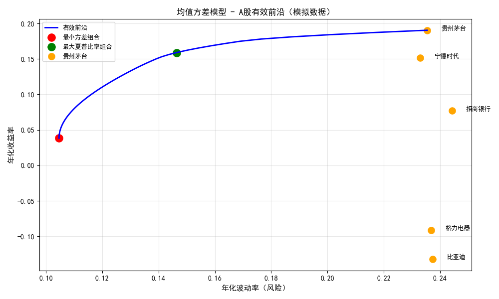
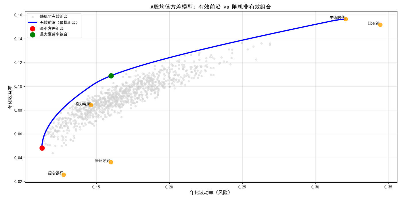
plt.plot(target_vols, target_returns, 'b-', linewidth=2, label='有效前沿')
# 标注最小方差组合（红色）
plt.scatter(min_vol_vol, min_vol_return, c='red', s=120, label='最小方差组合')
# 标注最大夏普比率组合（绿色）
plt.scatter(max_sharpe_vol, max_sharpe_return, c='green', s=120, label='最大夏普比率组合')

# 标注单个资产（橙色）
for i, ticker in enumerate(tickers):
    asset_vol = np.sqrt(cov.iloc[i, i])  # 单资产波动率
    asset_ret = mu[i]                    # 单资产收益率
    plt.scatter(asset_vol, asset_ret, c='orange', s=90, label=ticker_names[i] if i==0 else "")
    plt.text(asset_vol + 0.005, asset_ret, ticker_names[i], fontsize=9)

# 图表样式设置
plt.xlabel('年化波动率（风险）', fontsize=11)
plt.ylabel('年化收益率', fontsize=11)
plt.title('均值方差模型 - A股有效前沿（模拟数据）', fontsize=12)
plt.legend(loc='upper left', fontsize=9)
plt.grid(True, alpha=0.3)
plt.tight_layout()
plt.show()

# ====================== 4. 输出结果 ======================
print("="*40)
print("均值方差模型计算结果（A股模拟数据）")
print("="*40)

print("\n【最小方差组合】（风险最低）")
print("-"*30)
for ticker, weight in zip(tickers, min_vol_weights):
    print(f"{name_map[ticker]} ({ticker}): {weight:.2%}")
print(f"组合年化收益：{min_vol_return:.2%}")
print(f"组合年化波动率：{min_vol_vol:.2%}")

print("\n【最大夏普比率组合】（风险调整收益最高）")
print("-"*30)
for ticker, weight in zip(tickers, max_sharpe_weights):
    print(f"{name_map[ticker]} ({ticker}): {weight:.2%}")
print(f"组合年化收益：{max_sharpe_return:.2%}")
print(f"组合年化波动率：{max_sharpe_vol:.2%}")
print(f"组合夏普比率：{(max_sharpe_return - risk_free_rate)/max_sharpe_vol:.2f}")